# Random Forests for Change Point Detection
Change point detection aims to identify structural breaks in the probability
distribution of a time series. Existing methods either assume a parametric model for
within-segment distributions or are based on ranks or distances and thus fail in
scenarios with a reasonably large dimensionality.
`changeforest` implements a classifier-based algorithm that consistently estimates
change points without any parametric assumptions, even in high-dimensional scenarios.
It uses the out-of-bag probability predictions of a random forest to construct a
classifier log-likelihood ratio that gets optimized using a computationally feasible two-step
method.
See [1] for details.
`changeforest` is available as rust crate, a Python package (on
[`PyPI`](https://pypi.org/project/changeforest/) and
[`conda-forge`](https://anaconda.org/conda-forge/changeforest)),
and an R package (on [`conda-forge`](https://anaconda.org/conda-forge/r-changeforest)
, linux and MacOS only). See below for their respective user guides.
## Python
### Installation
To install from `conda-forge` (recommended), run
```bash
conda install -c conda-forge changeforest
```
To install from `PyPI`, run
```bash
pip install changeforest
```
### Example
In the following example, we perform random forest-based change point detection on
a simulated dataset with `n=600` observations and covariance shifts at `t=200, 400`.
```python
In [1]: import numpy as np
...:
...: Sigma = np.full((5, 5), 0.7)
...: np.fill_diagonal(Sigma, 1)
...:
...: rng = np.random.default_rng(12)
...: X = np.concatenate(
...: (
...: rng.normal(0, 1, (200, 5)),
...: rng.multivariate_normal(np.zeros(5), Sigma, 200, method="cholesky"),
...: rng.normal(0, 1, (200, 5)),
...: ),
...: axis=0,
...: )
```
The simulated dataset `X` coincides with the _change in covariance_ (CIC) setup
described in [1]. Observations in the first and last segments are independently drawn
from a standard multivariate Gaussian distribution. Observations in the second segment
are i.i.d. normal with mean zero and unit variance, but with a covariance of ρ = 0.7
between coordinates. This is a challenging scenario.
```python
In [2]: from changeforest import changeforest
...:
...: result = changeforest(X, "random_forest", "bs")
...: result
Out[2]:
best_split max_gain p_value
(0, 600] 400 14.814 0.005
¦--(0, 400] 200 59.314 0.005
¦ ¦--(0, 200] 6 -1.95 0.67
¦ °--(200, 400] 393 -8.668 0.81
°--(400, 600] 412 -9.047 0.66
In [3]: result.split_points()
Out[3]: [200, 400]
```
`changeforest` correctly identifies the change points at `t=200` and `t=400`. The
`changeforest` function returns a `BinarySegmentationResult`. We use its `plot` method
to investigate the gain curves maximized by the change point estimates:
```python
In [4]: result.plot().show()
```
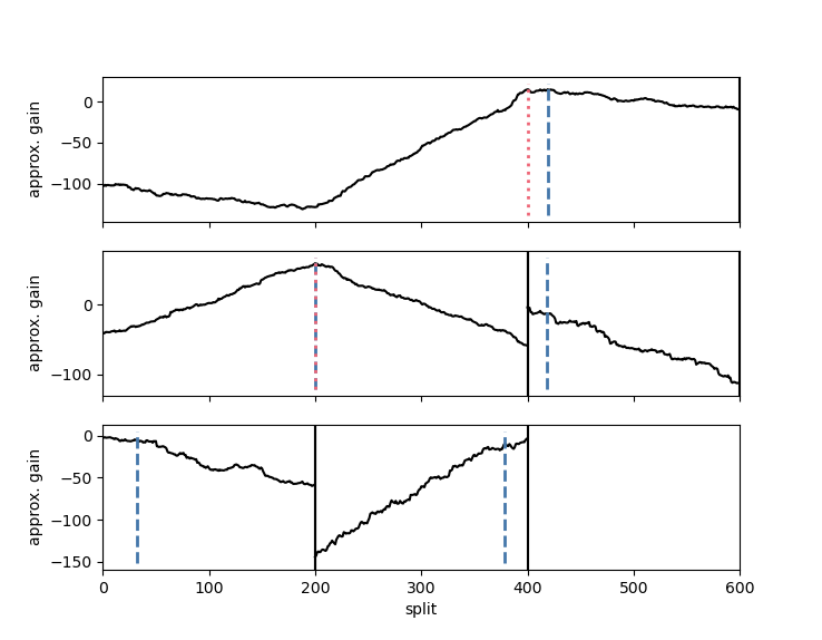
Change point estimates are marked in red.
For `method="random_forest"` and `method="knn"`, the `changeforest` algorithm uses a two-step approach to
find an optimizer of the gain. This fits a classifier for three split candidates
at the segment's 1/4, 1/2 and 3/4 quantiles, computes approximate gain curves using
the resulting classifier log-likelihood ratios and selects the overall optimizer as a second guess.
We can investigate the gain curves from the optimizer using the `plot` method of `OptimizerResult`.
The initial guesses are marked in blue.
```python
In [5]: result.optimizer_result.plot().show()
```
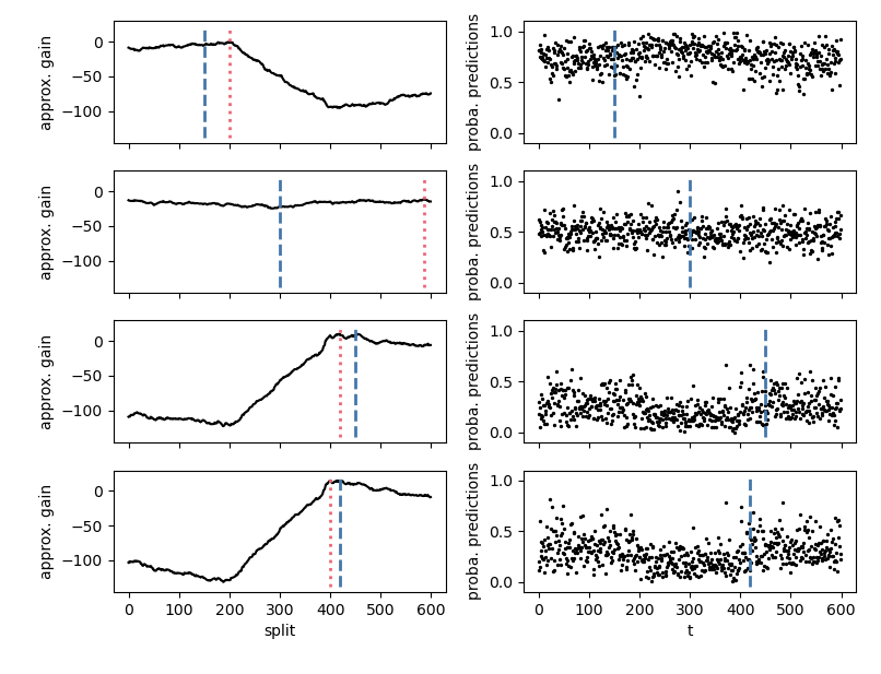
One can observe that the approximate gain curves are piecewise linear, with maxima
around the true underlying change points.
The `BinarySegmentationResult` returned by `changeforest` is a tree-like object with attributes
`start`, `stop`, `best_split`, `max_gain`, `p_value`, `is_significant`, `optimizer_result`, `model_selection_result`, `left`, `right` and `segments`.
These can be interesting to investigate the output of the algorithm further.
The `changeforest` algorithm can be tuned with hyperparameters. See
[here](https://github.com/mlondschien/changeforest/blob/287ac0f10728518d6a00bf698a4d5834ae98715d/src/control.rs#L3-L30)
for their descriptions and default values. In Python, the parameters can
be specified with the [`Control` class](https://github.com/mlondschien/changeforest/blob/b33533fe0ddf64c1ea60d0d2203e55b117811667/changeforest-py/changeforest/control.py#L1-L26),
which can be passed to `changeforest`. The following will build random forests with
50 trees:
```python
In [6]: from changeforest import Control
...: changeforest(X, "random_forest", "bs", Control(random_forest_n_estimators=50))
Out[6]:
best_split max_gain p_value
(0, 600] 416 7.463 0.01
¦--(0, 416] 200 43.935 0.005
¦ ¦--(0, 200] 193 -14.993 0.945
¦ °--(200, 416] 217 -9.13 0.085
°--(416, 600] 591 -12.07 1
```
The `changeforest` algorithm still detects change points at `t=200`, but is slightly off
with `t=416`.
Due to the nature of the change, `method="change_in_mean"` is unable to detect any
change points at all:
```python
In [7]: changeforest(X, "change_in_mean", "bs")
Out[7]:
best_split max_gain p_value
(0, 600] 589 8.625
```
## R
To install from `conda-forge`, run
```bash
conda install -c conda-forge r-changeforest
```
See [here](changeforest-r/Installing_R_packages_with_conda.md) for a detailed description
on installing the `changeforest` R package with `conda`.
### Example
In the following example, we perform random forest-based change point detection on
a simulated dataset with `n=600` observations and covariance shifts at `t=200, 400`.
```R
> library(MASS)
> set.seed(0)
> Sigma = matrix(0.7, nrow=5, ncol=5)
> diag(Sigma) = 1
> mu = rep(0, 5)
> X = rbind(
mvrnorm(n=200, mu=mu, Sigma=diag(5)),
mvrnorm(n=200, mu=mu, Sigma=Sigma),
mvrnorm(n=200, mu=mu, Sigma=diag(5))
)
```
The simulated dataset `X` coincides with the _change in covariance_ (CIC) setup
described in [1]. Observations in the first and last segments are independently drawn
from a standard multivariate Gaussian distribution. Observations in the second segment
are i.i.d. normal with mean zero and unit variance, but with a covariance of ρ = 0.7
between coordinates. This is a challenging scenario.
```R
> library(changeforest)
> result = changeforest(X, "random_forest", "bs")
> result
name best_split max_gain p_value is_significant
1 (0, 600] 410 13.49775 0.005 TRUE
2 ¦--(0, 410] 199 61.47201 0.005 TRUE
3 ¦ ¦--(0, 199] 192 -22.47364 0.955 FALSE
4 ¦ °--(199, 410] 396 11.50559 0.190 FALSE
5 °--(410, 600] 416 -23.52932 0.965 FALSE
> result$split_points()
[1] 199 410
```
`changeforest` correctly identifies the change point around `t=200` but is slightly
off at `t=410`. The `changeforest` function returns an object of class `binary_segmentation_result`.
We use its `plot` method to investigate the gain curves maximized by the change point estimates:
```R
> plot(result)
```
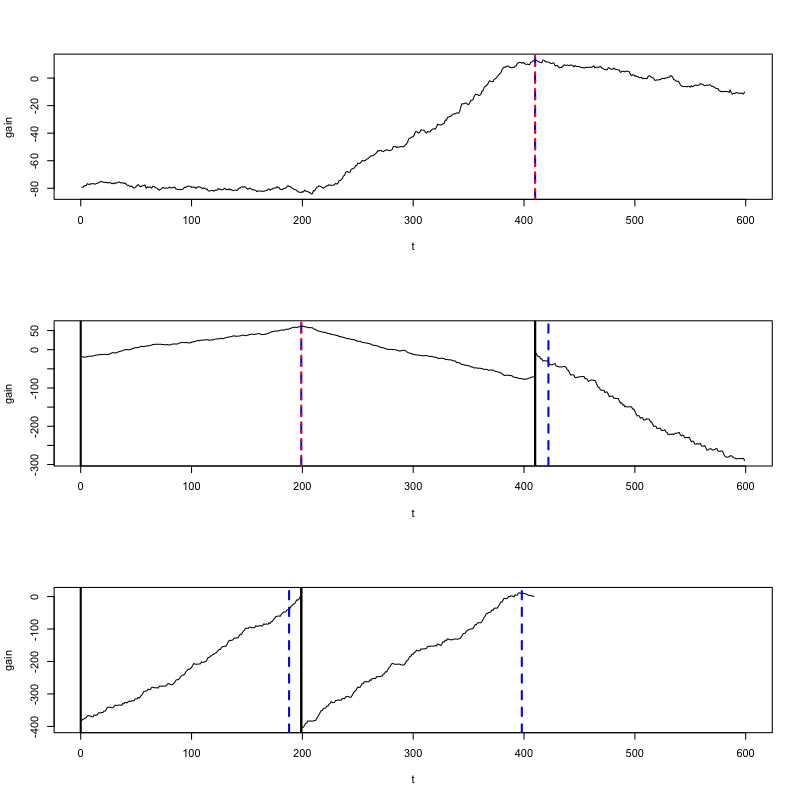
Change point estimates are marked in red.
For `method="random_forest"` and `method="knn"`, the `changeforest` algorithm uses a two-step approach to
find an optimizer of the gain. This fits a classifier for three split candidates
at the segment's 1/4, 1/2 and 3/4 quantiles computes approximate gain curves using
the resulting classifier log-likelihood ratios and selects the overall optimizer as a second guess.
We can investigate the gain curves from the optimizer using the `plot` method of `optimizer_result`.
The initial guesses are marked in blue.
```R
> plot(result$optimizer_result)
```
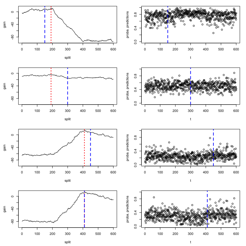
One can observe that the approximate gain curves are piecewise linear, with maxima
around the true underlying change points.
The `binary_segmentation_result` object returned by `changeforest` is a tree-like object with attributes
`start`, `stop`, `best_split`, `max_gain`, `p_value`, `is_significant`, `optimizer_result`, `model_selection_result`, `left`, `right` and `segments`.
These can be interesting to investigate the output of the algorithm further.
The `changeforest` algorithm can be tuned with hyperparameters. See
[here](https://github.com/mlondschien/changeforest/blob/287ac0f10728518d6a00bf698a4d5834ae98715d/src/control.rs#L3-L30)
for their descriptions and default values. In R, the parameters can
be specified with the `Control` class,
which can be passed to `changeforest`. The following will build random forests with
20 trees:
```R
> changeforest(X, "random_forest", "bs", Control$new(random_forest_n_estimators=20))
name best_split max_gain p_value is_significant
1 (0, 600] 15 -6.592136 0.010 TRUE
2 ¦--(0, 15] 6 -18.186534 0.935 FALSE
3 °--(15, 600] 561 -4.282799 0.005 TRUE
4 ¦--(15, 561] 116 -8.084126 0.005 TRUE
5 ¦ ¦--(15, 116] 21 -17.780523 0.130 FALSE
6 ¦ °--(116, 561] 401 11.782002 0.005 TRUE
7 ¦ ¦--(116, 401] 196 22.792401 0.150 FALSE
8 ¦ °--(401, 561] 554 -16.338703 0.800 FALSE
9 °--(561, 600] 568 -5.230075 0.120 FALSE
```
The `changeforest` algorithm still detects the change point around `t=200` but also
returns false positives.
Due to the nature of the change, `method="change_in_mean"` is unable to detect any
change points at all:
```R
> changeforest(X, "change_in_mean", "bs")
name best_split max_gain p_value is_significant
1 (0, 600] 498 17.29389 NA FALSE
```
## References
[1] M. Londschien, P. Bühlmann and S. Kovács (2023). "Random Forests for Change Point Detection" Journal of Machine Learning Research