polyfit
| Crates.io | polyfit |
| lib.rs | polyfit |
| version | 0.10.1 |
| created_at | 2026-01-13 19:16:56.573238+00 |
| updated_at | 2026-01-23 17:06:02.791212+00 |
| description | Because you don't need to be able to build a powerdrill to use one safely |
| homepage | |
| repository | https://github.com/rscarson/polyfit |
| max_upload_size | |
| id | 2040986 |
| size | 5,057,656 |
 Richard Carson (rscarson)
documentation
README
Polyfit
Because you don't need to be able to build a powerdrill to use one safely

![]()

Statistics is hard, and linear regression is made entirely out of footguns; Curve fitting might be simple in theory, but there sure is a LOT of theory.
This library is designed for developers who need to make use of the plotting or predictive powers of a curve fit without needing to worry about Huber loss, D'Agostino, or what on earth a kurtosis is
I provide a set a tools designed to help you:
- Select the right kind (basis) of polynomial for your data
- Automatically determine the optimal degree of the polynomial
- Make predictions, detect outliers, and get confidence values based on it
- Write easy to understand tests to confirm function
- Tests even plot the data and functions for you on failure! (
plottingfeature)
- Tests even plot the data and functions for you on failure! (
I support:
-
Functions and fits generic over floating point type and 11 choices of polynomial basis
- Monomial
- Orthogonal bases: Chebyshev (1st, 2nd, and 3rd forms), Legendre, Hermite (Physicists' and Probabilists'), Laguerre
- Fourier
- Logarithmic
-
Human-readable display of polynomial euations
-
Symbolic calculus (differentiation, integration, critical points) for most bases
-
Orthogonal basis specific tools (smoothness, coefficient energies, spectral energy truncation, orthogonal projection)
-
A suite of statistical tests to validate fit quality (
testmodule).- Tests include r², residual normality, homoscedasticity, autocorrelation, and more
- All tests generate plots on failure if the
plottingfeature is enabled
-
Data transformation tools (
transformsmodule) to add noise, scale, shift, and normalize data -
A library of statistical tools (
statisticsmodule) to help you understand your data -
Comprehensive engineering-focused documentation with examples and explanations, so you don't need a statistics degree to understand it
Crate features:
plotting- (default: NO) Enables plotting support usingplotters- All
assert_*macros in the testing library will generate plots on failure - The [
plot!] macro is available to generate plots of fits and polynomials - The [
plotting::Plot] type is available for more customized plots
- All
transforms- (default: YES) Enables data transformation tools- The [
transforms] module is available, which includes tools to add noise, scale, shift, and normalize data - The [
transforms::ApplyNoise] trait is available to add noise to data (Gaussian, Poisson, Impulse, Correlated, Salt & Pepper) - The [
transforms::ApplyScale] trait is available to scale data (Shift, Linear, Quadratic, Cubic) - The [
transforms::ApplyNormalization] trait is available to normalize data (Domain, Clip, Mean, zscore)
- The [
parallel- (default: NO) Enables parallel processing usingrayon- [
CurveFit::new_auto] uses parallel processing to speed up fitting when this feature is enabled - All curve fits can use a faster solver for large enough datasets when this feature is enabled
- [
The simplest use-case is to find a mathematical function to help approximate a set of data:
//
// Load data from a file
let data = include_str!("../examples/sample_data.json");
let data: Vec<(f64, f64)> = serde_json::from_str(data).unwrap();

//
// Now we can create a curve fit to this data
//
// `ChebyshevFit` is a type alias for `CurveFit<ChebyshevBasis>`
// `ChebyshevBasis` is a robust choice for many types of data; It's more numerically stable and performs better at higher degrees
// It is one of several bases available, each with their own strengths and weaknesses. `basis_select!` can help you choose the best one for your data
let fit = ChebyshevFit::new_auto(
    &data,                 // The data to fit to
    DegreeBound::Relaxed,  // How picky we are about the degree of the polynomial (See [`statistics::DegreeBound`])
    &Aic                   // The method used to score the fit quality (See [`crate::score`])
).expect("Failed to create fit");

//
// Of course if we don't test our code, how do we know it works - please don't assume I remembered all the edge cases
// If these assertion fail, a plot will be generated showing you exactly what went wrong!
//

// Here we test using r_squared, which is a measure of how well the curve explains how wiggly the data is
// An r_squared of 1.0 is a perfect fit
assert_r_squared!(fit);

// Here we check that the residuals (the difference between the data and the fit) are normally distributed
// Think of it like making sure the errors are random, not based on some undiscovered pattern
assert_residuals_normal!(fit);
Features
Built for developers, not statisticians
The crate is designed to be easy to use for developers who need to make use of curve fitting without needing to understand all the underlying statistics.
- Sensible defaults are provided for all parameters
- The most common use-cases are covered by simple functions and macros
- All documentation includes examples, explanations of parameters, and assumes zero prior knowledge of statistics
- API is designed to guide towards best practices, while being flexible enough to allow advanced users to customize behavior as needed
- Includes a suite of testing tools to bridge the gap between statistical rigour and engineering pragmatism
Hot-swappable Polynomial Basis
A polynomial basis is a sum of solving a function, called a basis function, multiplied by a coefficient:
y(x) = c1*b1(x) + c2*b2(x) + ... + cn*bn(x)
The basis determines what the basis functions b1, b2, ..., bn are. The choice of basis has massive implications for the shape of the curve,
the numerical stability of the fit, and how well it fits!
The crate includes a variety of polynomial bases to choose from, each with their own strengths and weaknesses.
[Polynomial] and [CurveFit] are generic over the basis, so you can easily swap them out to see which works best for your data:
- Monomial - Simple and intuitive, but can be numerically unstable for high degrees or wide x-ranges
- Chebyshev - More numerically stable than monomials, and can provide better fits for certain types of data
- Legendre - Orthogonal polynomials that can provide good fits for certain types of data
- Hermite (Physicists' and Probabilists') - Useful for data that is normally distributed
- Laguerre - Useful for data that is exponentially distributed
- Fourier - Useful for periodic data
I also include [basis_select!], a macro that will help you choose the best basis for your data.
- It does an automatic fit for each basis I support, and scores them using the method of your choice.
- It will show and plot out the best 3
- Use it a few times will real data and see which basis seems to consistently come out on top for your use-case
This table gives hints at which basis to choose based on the characteristics of your data:
| Basis Name | Handles Curves Well | Repeating Patterns | Extremes / Outliers | Growth/Decay | Best Data Shape / Domain |
|---|---|---|---|---|---|
| Monomial | Poor | No | No | Poor | Any simple trend |
| Chebyshev | Good | No | No | Poor | Smooth curves, bounded |
| Legendre | Fair | No | No | Poor | Smooth curves, bounded |
| Hermite | Good | No | Yes | Yes | Bell-shaped, any range |
| Laguerre | Good | No | Yes | Yes | Decaying, positive-only |
| Fourier | Fair | Yes | No | Poor | Periodic signals |
| Logarithmic | Fair | No | Yes | Yes | Logarithmic growth |
The orthogonal bases (Chebyshev, Legendre, Hermite, Laguerre) are generally more numerically stable than monomials, and can often provide better fits for higher-degree polynomials.
They also unlock a few analytical tools that are not available other bases:
- [
CurveFit::smoothness] - A measure of how "wiggly" the curve is; useful for regularization and model selection - [
CurveFit::coefficient_energies] - A measure of how much each basis function contributes to the overall curve; useful for understanding the shape of the curve - [
Polynomial::spectral_energy_truncation] - A way to de-noise the curve by removing high-frequency components the don't contribute enough; useful for smoothing noisy data - [
Polynomial::project_orthogonal] - A way to project any function onto an orthogonal basis- I like to use this to convert Fourier fits into Chebyshev fits for noisy periodic data (see
examples/whats_an_orthogonal.rs)
- I like to use this to convert Fourier fits into Chebyshev fits for noisy periodic data (see
Calculus Support
Most built-in bases support differentiation and integration in some way, including built-in methods for definite integrals, and finding critical points.
- Many basis options implement calculus directly
- A few bases implement
IntoMonomialBasis, which allows them to be converted into a monomial basis for calculus operations - For logarithmic series, use [
Polynomial::project], which can be a good way to approximate over certain ranges
| Basis | Exact Root Finding | Derivative | Integral (Indefinite) | As Monomial |
|---|---|---|---|---|
| Monomial | Yes | Yes | Yes | Yes |
| Chebyshev (1st form) | Yes | Yes | No | Yes |
| Chebyshev (2nd/3rd) | Yes | Yes | Yes | No |
| Legendre | No | Yes | No | Yes |
| Laguerre | No | Yes | No | Yes |
| Hermite | No | Yes | No | Yes |
| Fourier (sin/cos) | No | Yes | Yes | No |
| Exponential (e^{λx}) | No | Yes | Yes | No |
| Logarithmic (ln^n x) | No | No | No | No |
Testing Library
The crate includes a set of macros designed to make it easy to write unit tests to validate fit quality. There are a variety of assertions available, from simple r² checks to ensuring that residuals are normally distributed.
If the plotting feature is enabled, any failed assertion will generate a plot showing you exactly what went wrong.
See [mod@test] for more details on all included tests
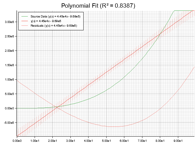
Plotting
If the plotting feature is enabled, you can use the [plot!] macro to generate plots of your fits and polynomials.
- Plots are saved as PNG files
- Fits include source data, confidence bands, and residuals
- If enabled, failed assertions in the testing library will automatically generate plots showing what went wrong
See [mod@plot] for more details
Transforms
If the transforms feature is enabled, you can use the tools in the [transforms] module to manipulate your data.
- Add noise for testing purposes
- Scale, shift, or normalize data
Human Readable Display
The crate includes a set of tools to help you display polynomials in a human readable format
- See the [
display] module for more details - All built-in basis options implement
PolynomialDisplayto give you a nicely formatted equation like: y(x) = 1.81x³ + 26.87x² - 1.00e3x + 9.03e3
Performance
The crate is designed to be fast and efficient, and includes benchmarks to help test that performance is linear with respect to the number of data points and polynomial degree.
A 3rd degree fit (1,000 points, Chebyshev basis) takes about 23µs in my benchmarks. Going up to 100,000 goes to about 4ms, which is roughly 100x the time for 1,000 points, as expected.
With parallelization turned on, a 100 million point fit for a 3rd degree Chebyshev took about 1.18s on my machine (8 cores @ 2.2GHz, 32GB RAM).
The same linear scaling can be seen with polynomial degree (1,000 points, Chebyshev basis); 11µs for degree 1, up to 44µs for degree 5.
Auto-fit is also reasonably fast; 1,000 points, Chebyshev basis, and 9 candidate degrees takes about 330µs, or 600µs with parallelization disabled.
There are also performance differences between bases; 1 - Chebyshev is the fastest, due to the stability of the matrix and the recurrence I use (~24µs for degree 3, 1,000 points) 2 - Hermite, Legendre, and Laguerre are fairly close to that (~30µs for degree 3, 1,000 points) 3 - Monomials perform worse than more stable bases (~53µs for degree 3, 1,000 points) 4 - Fourier and Logarithmic are around the same due to the trigonometric/logarithmic calculations (~57µs for degree 3, 1,000 points)
The benchmarks actually use my library to test that the scaling is linear - which I think is a pretty cool use-case:
let linear_fit = MonomialFit::new(&data, 1)?; // Create a linear fit (degree=1)
polyfit::assert_r_squared!(linear_fit);       // Assert that the linear fit explains the data well (r² > 0.9)

// If the assertion fails, a plot will be generated showing you exactly what went wrong
Raw benchmark results:
Benchmarking fit vs n (Chebyshev, Degree=3)
fit_vs_n/n=100                  [3.3817 µs 3.4070 µs 3.4363 µs]
fit_vs_n/n=1_000                [23.791 µs 23.926 µs 24.098 µs]
fit_vs_n/n=10_000               [302.99 µs 304.40 µs 306.01 µs]
fit_vs_n/n=100_000              [4.5086 ms 4.5224 ms 4.5376 ms]
fit_vs_n/n=1_000_000            [12.471 ms 12.592 ms 12.725 ms]
fit_vs_n/n=10_000_000           [115.49 ms 116.76 ms 118.07 ms]
fit_vs_n/n=100_000_000          [1.1768 s 1.1838 s 1.1908 s]

Benchmarking fit vs degree (Chebyshev, n=1000)
fit_vs_degree/Degree=1          [11.587 µs 11.691 µs 11.802 µs]
fit_vs_degree/Degree=2          [18.109 µs 18.306 µs 18.505 µs]
fit_vs_degree/Degree=3          [24.672 µs 24.954 µs 25.269 µs]
fit_vs_degree/Degree=4          [33.074 µs 33.206 µs 33.368 µs]
fit_vs_degree/Degree=5          [44.399 µs 44.887 µs 45.401 µs]
fit_vs_degree/Degree=10         [126.07 µs 127.26 µs 128.62 µs]
fit_vs_degree/Degree=20         [420.20 µs 423.44 µs 426.93 µs]

Benchmarking fit vs basis (Degree=3, n=1000)
fit_vs_basis/Monomial           [53.513 µs 53.980 µs 54.450 µs]
fit_vs_basis/Chebyshev          [24.307 µs 24.504 µs 24.710 µs]
fit_vs_basis/Legendre           [27.577 µs 80.104 µs 80.714 µs]
fit_vs_basis/Hermite            [30.496 µs 30.872 µs 31.321 µs]
fit_vs_basis/Laguerre           [31.146 µs 31.428 µs 31.734 µs]
fit_vs_basis/Fourier            [56.421 µs 56.985 µs 57.612 µs]

Benchmarking auto fit vs basis (n=1000, Candidates=9)
auto_fit_vs_basis/Monomial      [497.33 µs 500.27 µs 503.30 µs]
auto_fit_vs_basis/Chebyshev     [327.75 µs 329.67 µs 331.76 µs]
auto_fit_vs_basis/Legendre      [1.6993 ms 1.7061 ms 1.7128 ms]
auto_fit_vs_basis/Hermite       [337.65 µs 339.90 µs 342.44 µs]
auto_fit_vs_basis/Laguerre      [428.36 µs 431.26 µs 434.09 µs]
auto_fit_vs_basis/Fourier       [710.46 µs 713.07 µs 715.85 µs]
auto_fit_vs_basis/Logarithmic   [525.36 µs 528.21 µs 531.10 µs]
For transparency I ran the same benchmarks in numpy (benches/numpy_bench.py):
- They use 1,000points and Chebyshev basis for comparison. n tests are with degree 3
fit_vs_n/n=100         [465.15µs]
fit_vs_n/n=1000        [204.68µs]
fit_vs_n/n=10000       [953.67µs]
fit_vs_n/n=100000      [9847.16µs]

fit_vs_degree/degree=1 [122.67µs]
fit_vs_degree/degree=2 [158.31µs]
fit_vs_degree/degree=3 [198.84µs]
fit_vs_degree/degree=4 [243.07µs]
fit_vs_degree/degree=5 [510.57µs]
More Examples
Oh no! I have some data but I need to try and predict some other value!
//
// I don't have any real data, so I'm still going to make some up!
// `function!` is a macro that makes it easy to define polynomials for testing
// `apply_poisson_noise` is part of the `transforms` module, which provides a set of tools for manipulating data
polyfit::function!(f(x) = 2 x^2 + 3 x - 5);
let synthetic_data = f.solve_range(0.0..=100.0, 1.0).apply_poisson_noise(Strength::Absolute(0.1), None);

//
// Now we can create a curve fit to this data
// Monomials don't like high degrees, so we will use a more conservative degree bound
// `Monomials` are the simplest polynomial basis, and the one most people are familiar with, it looks like `1x^2 + 2x + 3`
let fit = MonomialFit::new_auto(&synthetic_data, DegreeBound::Conservative, &Aic).expect("Failed to create fit");

//
// Now we can make some predictions!
//

let bad_and_silly_prediction = fit.y(150.0); // This is outside the range of the data, so it is probably nonsense
                                             // Fits are usually only valid within the range of the data they were created from
                                             // Violating that is called extrapolation, which we generally want to avoid
                                             // This will return an error!

let bad_prediction_probably = fit.as_polynomial().y(150.0); // This is outside the range of the data, but you asked for it specifically
                                                            // Unlike a CurveFit, a Polynomial is just a mathematical function - no seatbelts
                                                            // This will return a value, but it is probably nonsense

let good_prediction = fit.y(50.0); // This is within the range of the data, so it is probably reasonable
                                   // This will return Ok(value)

//
// Maybe we need to make sure our predictions are good enough
// A covariance matrix sounds terrifying. Because it is.
// Which is why I do it for you - covariance matrices measure uncertainty about your fit
// They can be used to calculate confidence intervals for predictions
// They can also be used to find outliers in your data
let covariance = fit.covariance().expect("Failed to calculate covariance");
let confidence_band = covariance.confidence_band(
    50.0,                          // Confidence band for x=50
    Confidence::P95,               // Find the range where we expect 95% of points to fall within
    Some(Tolerance::Variance(0.1)) // Tolerate some extra noise in the data (10% of variance of the data, in this case)
).unwrap(); // 95% confidence band
println!("I am 95% confident that the true value at x=50.0 is between {} and {}", confidence_band.min(), confidence_band.max());
Oh dear! I sure do wish I could find which pieces of data are outliers!
//
// I still don't have any real data, so I'm going to make some up! Again!
polyfit::function!(f(x) = 2 x^2 + 3 x - 5);
let synthetic_data = f.solve_range(0.0..=100.0, 1.0).apply_poisson_noise(Strength::Absolute(0.1), None);

//
// Let's add some outliers
// Salt and pepper noise is a simple way to do this; She's good n' spiky
// We will get nice big jumps of +/- 50 in 5% of the data points
let synthetic_data_with_outliers = synthetic_data.apply_salt_pepper_noise(0.05, Strength::Absolute(-50.0), Strength::Absolute(50.0), None);

//
// Now we can create a curve fit to this data, like before
let fit = MonomialFit::new_auto(&synthetic_data_with_outliers, DegreeBound::Conservative, &Aic).expect("Failed to create fit");

//
// Now we can find the outliers!
// These are the points that fall outside the 95% confidence interval
// This means that they are outside the range where we expect 95% of the data to fall
// The `Some(0.1)` means we tolerate some noise in the data, so we don't flag points that are just a little bit off
// The noise tolerance is a fraction of the variance of the data (10% in this case)
//
// If we had a sensor that specified a tolerance of ±5 units, we could use `Some(Tolerance::Absolute(5.0))` instead
// If we had a sensor that specified a tolerance of 10% of the reading, we could use `Some(Tolerance::Measurement(0.1))` instead
let outliers = fit.covariance().unwrap().outliers(Confidence::P95, Some(Tolerance::Variance(0.1))).unwrap();