simple_moving_average
| Crates.io | simple_moving_average |
| lib.rs | simple_moving_average |
| version | 1.0.2 |
| created_at | 2021-09-20 12:44:30.471628+00 |
| updated_at | 2024-02-07 08:20:08.874403+00 |
| description | Library of simple moving average (SMA) algorithms |
| homepage | |
| repository | https://github.com/oskargustafsson/moving_average |
| max_upload_size | |
| id | 453994 |
| size | 46,118 |
documentation
README
simple_moving_average
This crate provides several algorithms for calculating the simple moving average (SMA) of a series of data samples. SMAs are commonly used to implement low-pass filters, the second-most useful filter type, bested only by coffee filters.
All algorithms implement the [SMA] trait, which provides an implementation-agnostic interface. The interface is generic over sample type, meaning that any type that supports addition and division by a scalar can be averaged. This includes most primitive numeric types (f32, u32, ...), Duration and many third party math library (e.g. nalgebra, euclid, cgmath, ...) vector and matrix types.
Project status
The library is actively used, feature complete, fully tested and there are no known bugs. It can be considered production ready, but it is not actively developed, as there are no obvious needs motivating it. Bug reports, feature requests and pull requests are welcome through GitHub.
Examples
Scalars
let mut ma = SumTreeSMA::<_, f32, 2>::new(); // Sample window size = 2
ma.add_sample(1.0);
ma.add_sample(2.0);
ma.add_sample(3.0);
assert_eq!(ma.get_average(), 2.5); // = (2 + 3) / 2
Vectors
let mut ma = NoSumSMA::<_, f64, 2>::new();
ma.add_sample(Vector3::new(1.0, 2.0, 3.0));
ma.add_sample(Vector3::new(-4.0, -2.0, -1.0));
assert_eq!(ma.get_average(), Vector3::new(-1.5, 0.0, 1.0));
Durations
let mut ma = SingleSumSMA::<_, _, 10>::from_zero(Duration::ZERO);
loop {
	let instant = Instant::now();
	// [ application code ]
	ma.add_sample(instant.elapsed());
	dbg!("Average iteration duration: {}", ma.get_average());
	# break;
}
Algorithm implementations
One way to achieve good performance when calculating simple moving averages is to cache previous calculations, specifically the sum of the samples currently in the sample window. Caching this sum has both pros and cons, which is what motivates the three different implementations presented below.
| Implementation | Add sample | Get average | Caveat |
|---|---|---|---|
| [NoSumSMA] | O(1) |
O(N) |
- |
| [SingleSumSMA] | O(1) |
O(1) |
Accumulates floating point rounding errors. |
| [SumTreeSMA] | O(log(N)) |
O(1) |
- |
N refers to the size of the sample window.
All implementations have O(N) space complexity. [NoSumSMA] and [SingleSumSMA] are completely
// backed by arrays, so they are by default stack allocated. [SumTreeSMA] stores some data in an
array, but its sum tree is stored in a Vec.
NoSumSMA
The most straightforward way of implementing a moving average is to not cache any sum at all, hence
the name if this implementation. The sum of all samples is calculated from scratch, at O(N) time
complexity (N being the sample window size), every time the average is requested.
When to use
- When the sample window size is so small that the samples summation cost is negligible.
- When new samples are written significantly more often than the average value is read.
SingleSumSMA
This implementation caches the sum of all samples in the sample window as a single value, leading to
O(1) time complexity for both writing new samples and reading their average. A problem with this
approach is that most floating point numbers can't be stored exactly, so every time a such a number
is added to the cached sum, there is a risk of accumulating a rounding error.
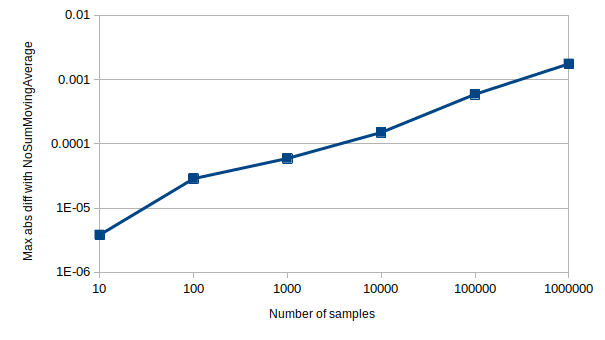
The magnitude of the accumulated error depends on many factors, including sample window size and sample distribution. Below is a visualization of how the absolute difference in average value between [SingleSumSMA] and [NoSumSMA] (which does not suffer from accumulated rounding errors) grows with the number of samples, for a typical window size and set of samples.
Sample type: f32, Sample window size: 10,
Sample distribution: Uniform[-100, 100]

Note: Both axes of the graph are logarithmic. The Y axis values represent the maximum differences found over 100 test runs.
One way to reduce the error is to use wider type, e.g. f64 instead of f32. The absolute error is
also less prominent when the samples lie near the interval [-1, 1], as that is where floating
point precision is at its highest.
When to use
- When sample values can be represented exactly in memory, in which case there is no downside to this approach. This is true for all primitive integer types and Duration.
- When performance is more important than numerical accuracy.
SumTreeSMA
There is a way of avoiding the accumulated floating point rounding errors, without having to re-calculate the whole samples sum every time the average value is requested. The downside though, is that it involves both math and binary trees:
A sum is the result of applying the binary and associative addition operation to a set of operands, which means that it can be represented as a binary tree of sums.
For example
(1) + (2) + (3) + (4) + (5) + (6) =
(1 + 2) + (3 + 4) + (5 + 6) =
(3) + (7) + (11) =
(3 + 7) + (11) =
(10) + (11) =
(10 + 11) =
(21)
can be represented as the following tree.
21
/ \
/ \
10 11
/ \ \
/ \ \
3 7 11
/ \ / \ / \
1 2 3 4 5 6
If one of the leaf nodes (i.e. samples) were to change, only the nodes comprising the direct
path between that leaf and the root need to be re-calculated, leading to log(N) calculations, N
being the window size. This is exactly what happens when a sample is added; the oldest sample gets
replaced with the new sample and sum tree leaf node corresponding to the oldest sample is updated
with the new sample value.
One existing leaf node (i.e. sample value) is always re-read when updating that leaf node's neighbor, meaning that after N samples have been added, all the leaf nodes have been re-read. This is what keeps the floating point rounding error from accumulating.
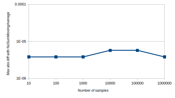
Author's note: If anyone has the brains and will to prove this formally, they are most welcome to submit a PR. In the mean time, there is a unit test that empirically proves that the rounding error does not accumulate. Part of that test's output data is visualized in the graph below, showing no accumulated rounding errors when compared with [NoSumSMA].

When to use
-
In most cases where floating point data is involved, unless writes are much more common than reads.
License
MIT